CS189 Assignment 3#

项目描述#

这个lab主要聚焦于实现优化器和反向传播(逐项求导), 和CS336的lab1当中的实现类似

例子: 多元微分#

我们用课程组给出的例子来复习一下多元微分

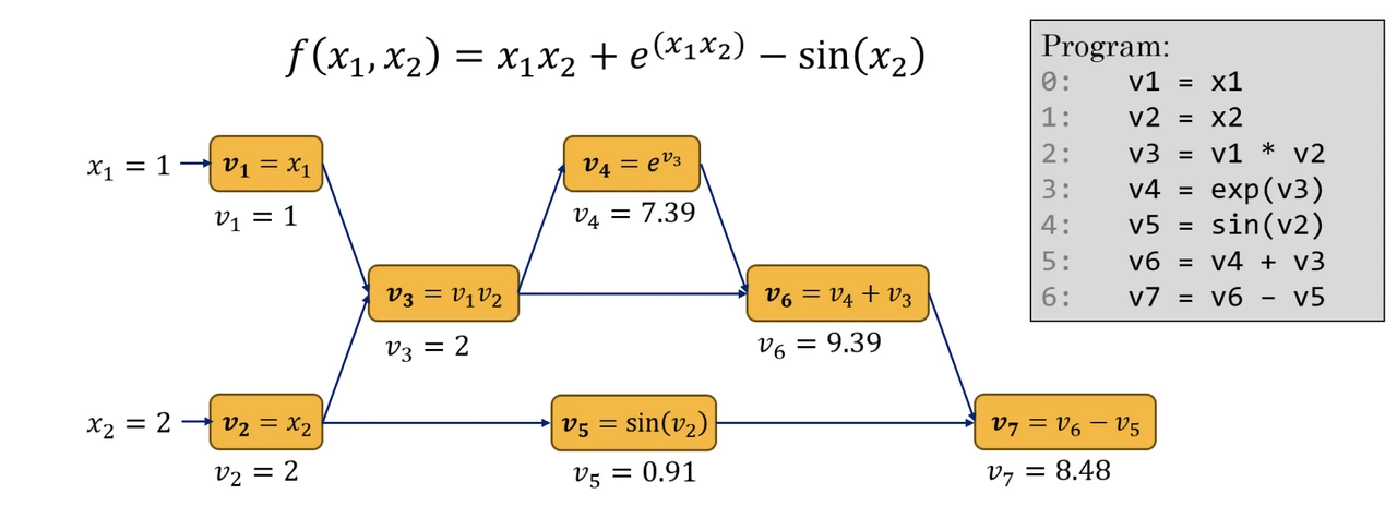
中间变量是从v1到v7

\frac{\partial v_7}{\partial v_7} = 1

v_7 = v_6 - v_5 \implies \frac{\partial v_7}{\partial v_6} = 1, \quad \frac{\partial v_7}{\partial v_5} = -1

v_6 = v_4 + v_3 \implies \frac{\partial v_6}{\partial v_4} = 1, \quad \frac{\partial v_6}{\partial v_3} = 1

\frac{\partial v_7}{\partial v_4} = \frac{\partial v_7}{\partial v_6} \cdot \frac{\partial v_6}{\partial v_4} = 1 \cdot 1 = 1

\frac{\partial v_7}{\partial v_3} = \frac{\partial v_7}{\partial v_6} \cdot \frac{\partial v_6}{\partial v_3}

\frac{\partial v_6}{\partial v_3} = \frac{\partial v_6}{\partial v_3} + \frac{\partial v_6}{\partial v_4} \cdot \frac{\partial v_4}{\partial v_3} = 1 + e^{v_3}

\frac{\partial v_7}{\partial v_3} = 1 + e^{v_3}

\frac{\partial v_7}{\partial v_2} = \frac{\partial v_7}{\partial v_6} \cdot \frac{\partial v_6}{\partial v_2} + \frac{\partial v_7}{\partial v_5} \cdot \frac{\partial v_5}{\partial v_2} = \frac{\partial v_6}{\partial v_2} - \frac{\partial v_5}{\partial v_2} = \frac{\partial v_6}{\partial v_2} - \cos(v_2)

\frac{\partial v_6}{\partial v_2} = \frac{\partial v_6}{\partial v_4} \cdot \frac{\partial v_4}{\partial v_2} + \frac{\partial v_6}{\partial v_3} \cdot \frac{\partial v_3}{\partial v_2} = \frac{\partial v_4}{\partial v_2} + \frac{\partial v_3}{\partial v_2} = \frac{\partial v_4}{\partial v_3} \cdot \frac{\partial v_3}{\partial v_2} + v_1 = e^{v_3} \cdot v_1 + v_1

\frac{\partial v_7}{\partial v_1} = \frac{\partial v_7}{\partial v_6} \cdot \frac{\partial v_6}{\partial v_1} = \frac{\partial v_6}{\partial v_1} = \frac{\partial v_6}{\partial v_4} \cdot \frac{\partial v_4}{\partial v_1} + \frac{\partial v_6}{\partial v_3} \cdot \frac{\partial v_3}{\partial v_1} = \frac{\partial v_4}{\partial v_1} + \frac{\partial v_3}{\partial v_1} = \frac{\partial v_4}{\partial v_3} \cdot \frac{\partial v_3}{\partial v_1} + \frac{\partial v_3}{\partial v_1} \\ = e^{v_3} \cdot v_2 + v_2

所谓反向传播就是把每一次算出来的中间结果记住, 然后用链式法则一步步的向前求导,比如说最初的输入是x,y, 输出是z, 通过计算z对一大堆中间变量的偏导数, 最终计算得到

\frac{\partial z}{\partial x} \,\,and \,\, \frac{\partial z}{\partial y}

如果对上面的求偏导过程有疑问, 建议去看一看微积分(下)或者数学分析(三)

Problem 1#

既然要求微分, 首先要实现Tensor之间的运算, 注意到正如上面那个图所示, 我们需要三个类:

— class BearGrad 来给出一个可调用的函数, 根据上游梯度来计算下游梯度 — class BearParent 来记录图的边, 即每个节点的parent节点是什么 — class BearTensor 来提供各种基础运算, 例如加减乘除

@dataclass
class BearGrad:
    '''Stores how to compute the downstream gradient from the upstream gradient 
    - `op_str` is just a string describing the operation; you don't need to use this for this HW, but it may help in debugging if you print out what operations create your computation graph.
    - `fn` is a function that takes in the upstream loss gradient and outputs the loss gradient that should be passed downstream. This essentially applies the chain rule at the current node in the computation graph.
    '''
    fn: callable
    op_str: str | None = None

python

这是梯度计算器, fn函数用于计算下游梯度, op_str用来描述这个操作

例如我们有一个中间变量c = a + b

a ────┐
      ├──→ c = a + b ──→ 上游梯度 (∂L/∂c)
b ────┘

plaintext

这个BearGrad类需要给出L对a和b的偏导数, 即∂L/∂a和∂L/∂b, 这种情况下fn大概是一个加法的梯度函数:

def add_grad_fn(upstream_grad):
    # ∂L/∂a = ∂L/∂c * ∂c/∂a = ∂L/∂c * 1
    # ∂L/∂b = ∂L/∂c * ∂c/∂b = ∂L/∂c * 1
    return upstream_grad  # 因为 ∂c/∂a = 1

python

父节点追踪器:

@dataclass
class BearParent:
    '''This class represents a parent of a node; a node must track its parents so that it knows who to propagate its gradients to.
    - `grad` is the `BearGrad` object for this parent; we can apply the `fn` from this to compute the gradient that should be passed downstream.
    - `parent` is the `BearTensor` object for the parent
    '''
    parent: BearTensor
    grad: BearGrad

    def __hash__(self):
        return id(self)

    def __eq__(self, other):
        return self is other

python

要记录父节点和grad, grad代表了”在已知上游梯度的情况下, 如何算出下游梯度”

顺便解释一下类装饰器@dataclass, 用了这个装饰器就会自动生成一些方法, 比如:

__init__
__repr__ (字符串表示)
__eq__ (相等比较)

plaintext

等等

class BearTensor:
    '''`BearTensor`: This represents a node in our computation graph
    - `value` is the underlying data in the Tensor; this is computed during the forward pass
    - `parents` keeps track of the parents in the computation graph to whom we pass our gradient to
    - `adjoint` is the gradient (the transpose of it technically) that we compute in the backward pass
    '''
    def __init__(self, name: str, value: np.ndarray, parents: list[BearParent] | None = None):
        self.name = name
        self.value = value
        self.parents = parents if parents is not None else []
        self.adjoint: float | np.ndarray = 0.0

python

我们要实现各种运算和相对于那种运算的梯度公式

- Addition (`__add__`)
- Subtraction (`__sub__`)
- Multiplication (`__mul__`)
- Power (`__pow__`)
- Matrix multiplication (`__matmul__`)
- Dot product (`dot`)
- Sum (`sum`)
- Mean (`mean`)
- ReLU (`relu`)
- Sigmoid (`sigmoid`)

plaintext

先来看__add__的实现, 这个运算要对self.value和other.value进行加法运算, 新BearTensor.value就是self.value + other.value

接下来思考这个问题: 返回的新的BearTensor的parents应该是什么?

return BearTensor(name=f"{self.name} + {other.name}", value=new_value, parents=parents)

python

新的parents应该有两个节点, 分别为self和other, 但是parent必须为BearParent类, 而构造这个类的时候需要两个参数: BearTensor和BearGrad, 显然BearTensor已经有了, BearGrad需要我们手动演算一下求导的函数

设有两个 Tensor:

$a$ : BearTensor, 值为 $a$
$b$ : BearTensor, 值为 $b$
$c = a + b$ : BearTensor, 值为 $c = a + b$

我们需要计算 $\frac{\partial L}{\partial a}$ 和 $\frac{\partial L}{\partial b}$ ，其中 $L$ 是最终损失函数：

\begin{align*} \frac{\partial L}{\partial a} = \frac{\partial L}{\partial c} \cdot \frac{\partial c}{\partial a} \\ \frac{\partial L}{\partial b} = \frac{\partial L}{\partial c} \cdot \frac{\partial c}{\partial b} \\ \frac{\partial c}{\partial a} = \frac{\partial (a + b)}{\partial a} = 1 \\ \frac{\partial c}{\partial b} = \frac{\partial (a + b)}{\partial b} = 1\\ \frac{\partial L}{\partial a} = \frac{\partial L}{\partial c} \cdot 1 = \frac{\partial L}{\partial c}\\ \frac{\partial L}{\partial b} = \frac{\partial L}{\partial c} \cdot 1 = \frac{\partial L}{\partial c} \end{align*}

换言之, 这里的两个下游梯度都等于传过来的上游梯度, 所以两个fn函数的返回值保持不变

    def __add__(self, other: BearTensor) -> BearTensor:
        if self.value.shape != other.value.shape:
            raise ValueError("Shapes must match")
        
        new_value = self.value + other.value

        def grad_fn(upstream_grad):
            return upstream_grad

        def grad_fn_other(upstream_grad):
            return upstream_grad

        parents=[
            BearParent(parent=self, grad=BearGrad(fn=grad_fn,op_str='text("add")')),
            BearParent(parent=other, grad=BearGrad(fn=grad_fn_other,op_str='text("add")'))
        ]

        return BearTensor(name=f"{self.name} + {other.name}", value=new_value, parents=parents)

python

减法也一样

\begin{align*} \frac{\partial L}{\partial a} = \frac{\partial L}{\partial c} \cdot \frac{\partial c}{\partial a} \\ \frac{\partial L}{\partial b} = \frac{\partial L}{\partial c} \cdot \frac{\partial c}{\partial b} \\ \frac{\partial c}{\partial a} = \frac{\partial (a - b)}{\partial a} = 1 \\ \frac{\partial c}{\partial b} = \frac{\partial (a - b)}{\partial b} = -1\\ \frac{\partial L}{\partial a} = \frac{\partial L}{\partial c} \cdot 1 = \frac{\partial L}{\partial c}\\ \frac{\partial L}{\partial b} = \frac{\partial L}{\partial c} \cdot -1 = -\frac{\partial L}{\partial c} \end{align*}

乘法

\begin{align*} \frac{\partial L}{\partial a} = \frac{\partial L}{\partial c} \cdot \frac{\partial c}{\partial a} \\ \frac{\partial L}{\partial b} = \frac{\partial L}{\partial c} \cdot \frac{\partial c}{\partial b} \\ \frac{\partial c}{\partial a} = \frac{\partial (a \cdot b)}{\partial a} = b \\ \frac{\partial c}{\partial b} = \frac{\partial (a \cdot b)}{\partial b} = a \\ \frac{\partial L}{\partial a} = \frac{\partial L}{\partial c} \cdot b \\ \frac{\partial L}{\partial b} = \frac{\partial L}{\partial c} \cdot a \end{align*}

    def __mul__(self, other: BearTensor) -> BearTensor:
        if self.value.shape != other.value.shape:
            raise ValueError("Shapes must match")
        
        new_value = self.value * other.value

        def grad_fn(upstream_grad):
            return other.value*upstream_grad
        
        def grad_fn_other(upstream_grad):
            return self.value*upstream_grad

        parents=[
            BearParent(parent=self, grad=BearGrad(fn=grad_fn,op_str='text("mul")')),
            BearParent(parent=other, grad=BearGrad(fn=grad_fn_other,op_str='text("mul")'))
        ]

        return BearTensor(name=f"{self.name} * {other.name}", value=new_value, parents=parents)

python

幂运算, 此时另外一个输入变成固定的数power, 记作n

\begin{align*} \frac{\partial L}{\partial a} = \frac{\partial L}{\partial c} \cdot \frac{\partial c}{\partial a} \\ \frac{\partial c}{\partial a} = \frac{\partial (a^n)}{\partial a} = n \cdot a^{n-1} \\ \frac{\partial L}{\partial a} = \frac{\partial L}{\partial c} \cdot n \cdot a^{n-1} \\ \end{align*}

    def __pow__(self, power: float) -> BearTensor:
        
        new_value=self.value**power

        def grad_fn(upstream_grad):
            return upstream_grad*power*self.value**(power-1)

        parents=[
            BearParent(parent=self, grad=BearGrad(fn=grad_fn,op_str='text("pow")'))
        ]

        return BearTensor(name=f"{self.name}**{power}", value=new_value, parents=parents)

python

矩阵乘法, 注意这里要用向量微积分

\begin{align*} \frac{\partial L}{\partial A} &: (m,n) \\ \frac{\partial L}{\partial C} &: (m,p) \\ C &= A \cdot B : (m,p) \\ A &: (m,n), \quad B : (n,p) \\[8pt] \frac{\partial L}{\partial A} &= \frac{\partial L}{\partial C} \cdot B^T \\ (m,n) &= (m,p) \cdot (p,n) \\[8pt] \frac{\partial L}{\partial B} &= A^T \cdot \frac{\partial L}{\partial C} \\ (n,p) &= (n,m) \cdot (m,p) \end{align*}

    def __matmul__(self, other: BearTensor) -> BearTensor:
        # This may be helpful to avoid shape mismatch errors
        def ensure_2d(x):
            '''If x is a scalar or 1-D, convert to 2-D'''
            x = np.asarray(x)
            if x.ndim == 0:          # scalar
                return x.reshape(1, 1)
            elif x.ndim == 1:        # vector
                return x.reshape(-1, 1)  # column vector convention
            else:                     # already 2D
                return x
        
        new_value=np.matmul(ensure_2d(self.value), ensure_2d(other.value))

        def grad_fn(upstream_grad):

            return np.matmul(upstream_grad,other.value.T)

        def grad_fn_other(upstream_grad):

            return np.matmul(self.value.T,upstream_grad)

        parents=[
            BearParent(parent=self, grad=BearGrad(fn=grad_fn,op_str='text("matmul")')),
            BearParent(parent=other, grad=BearGrad(fn=grad_fn_other,op_str='text("matmul")'))
        ]

        return BearTensor(name=f"{self.name} @ {other.name}", value=new_value, parents=parents)

python

记住向量求导的尺寸约定: 偏导数(矩阵)的尺寸保持为”分母”的尺寸, 比如 $\frac{\partial L}{\partial A}$ 的尺寸为 $(m,n)$ , 因为 $A$ 的尺寸为 $(m,n)$

点积运算

\begin{align*} c &= \mathbf{a} \cdot \mathbf{b} = \sum_{i=1}^n a_i b_i, \quad \mathbf{a}_{(n)}, \mathbf{b}_{(n)} \\[8pt] \frac{\partial c}{\partial \mathbf{a}} &= \mathbf{b} \\[6pt] \frac{\partial L}{\partial \mathbf{a}}_{(n)} &= \frac{\partial L}{\partial c}_{(1)} \cdot \mathbf{b}_{(n)} \\[12pt] \frac{\partial c}{\partial \mathbf{b}} &= \mathbf{a} \\[6pt] \frac{\partial L}{\partial \mathbf{b}}_{(n)} &= \frac{\partial L}{\partial c}_{(1)} \cdot \mathbf{a}_{(n)} \end{align*}

    def dot(self, other: BearTensor) -> BearTensor:
        if self.value.ndim != 1 or other.value.ndim != 1:
            raise ValueError("dot() only supports 1-D BearTensors (like torch.dot).")

        new_value=np.dot(self.value,other.value)

        new_value=np.array([new_value])
            
        def grad_fn(upstream_grad):

            return upstream_grad*other.value

        def grad_fn_other(upstream_grad):

            return upstream_grad*self.value

        parents=[
            BearParent(parent=self, grad=BearGrad(fn=grad_fn,op_str='text("dot")')),
            BearParent(parent=other, grad=BearGrad(fn=grad_fn_other,op_str='text("dot")'))
        ]

        return BearTensor(name=f"{self.name} @ {other.name}", value=new_value, parents=parents)

python

自求和

\begin{align*} s &= \sum_{i=1}^n x_i = \text{sum}(\mathbf{x}), \quad \mathbf{x}_{(n)} \implies s_{(1)} \\[8pt] \frac{\partial s}{\partial \mathbf{x}} &= \begin{bmatrix} 1 & 1 & \cdots & 1 \end{bmatrix}_{(n)} \\[6pt] \frac{\partial L}{\partial \mathbf{x}}_{(n)} &= \frac{\partial L}{\partial s}_{(1)} \cdot \mathbf{1}_{(n)} \end{align*}

    def sum(self) -> BearTensor:
        
        new_value=np.array([np.sum(self.value)])

        def grad_fn(upstream_grad):
            return np.ones_like(self.value)*upstream_grad

        parents=[
            BearParent(parent=self, grad=BearGrad(fn=grad_fn,op_str='text("sum")'))
        ]

        return BearTensor(name=f"sum({self.name})", value=new_value, parents=parents)

python

自平均运算

\begin{align*} \mu &= \text{mean}(\mathbf{x}) = \frac{1}{n} \sum_{i=1}^n x_i, \quad \mathbf{x}_{(n)} \implies \mu_{(1)} \\[8pt] \frac{\partial \mu}{\partial \mathbf{x}} &= \frac{1}{n} \begin{bmatrix} 1 & 1 & \cdots & 1 \end{bmatrix}_{(n)} \\[6pt] \frac{\partial L}{\partial \mathbf{x}}_{(n)} &= \frac{\partial L}{\partial \mu}_{(1)} \cdot \frac{1}{n} \cdot \mathbf{1}_{(n)} \end{align*}

    def mean(self) -> BearTensor:
        
        new_value=np.array([np.mean(self.value)])

        def grad_fn(upstream_grad):
            return np.ones_like(self.value)*upstream_grad/self.value.size

        parents=[
            BearParent(parent=self, grad=BearGrad(fn=grad_fn,op_str='text("mean")'))
        ]

        return BearTensor(name=f"mean({self.name})", value=new_value, parents=parents)

python

ReLU运算

\begin{align*} y &= \text{ReLU}(x) = \max(0, x) \\[8pt] \frac{\partial y}{\partial x} &= \begin{cases} 1 & \text{if } x > 0 \\ 0 & \text{if } x \leq 0 \end{cases} = \mathbb{1}(x > 0) \\[8pt] \frac{\partial L}{\partial x} &= \frac{\partial L}{\partial y} \cdot \frac{\partial y}{\partial x} = \frac{\partial L}{\partial y} \cdot \mathbb{1}(x > 0) \end{align*}

    def relu(self) -> BearTensor:
        
        new_value=np.maximum(0, self.value)

        def grad_fn(upstream_grad):
            return (self.value>0)*upstream_grad

        parents=[
            BearParent(parent=self, grad=BearGrad(fn=grad_fn,op_str='text("relu")'))
        ]

        return BearTensor(name=f"relu({self.name})", value=new_value, parents=parents)

python

注意这个求导在数学上是有瑕疵的, ReLU函数在0处并不可导

Sigmoid函数

\begin{align*} y &= \sigma(x) = \frac{1}{1 + e^{-x}} \\[8pt] \frac{dy}{dx} &= \sigma(x)(1 - \sigma(x)) = y(1 - y) \\[8pt] \frac{\partial L}{\partial x} &= \frac{\partial L}{\partial y} \cdot \frac{dy}{dx} = \frac{\partial L}{\partial y} \cdot y(1 - y) \end{align*}

    def sigmoid(self) -> BearTensor:
        
        new_value=1 / (1 + np.exp(-self.value))

        def grad_fn(upstream_grad):
            return upstream_grad*new_value*(1-new_value)

        parents=[
            BearParent(parent=self, grad=BearGrad(fn=grad_fn,op_str='text("sigmoid")'))
        ]

        return BearTensor(name=f"sigmoid({self.name})", value=new_value, parents=parents)

python

课程组给了一个链式图的demo绘图代码, 图如下

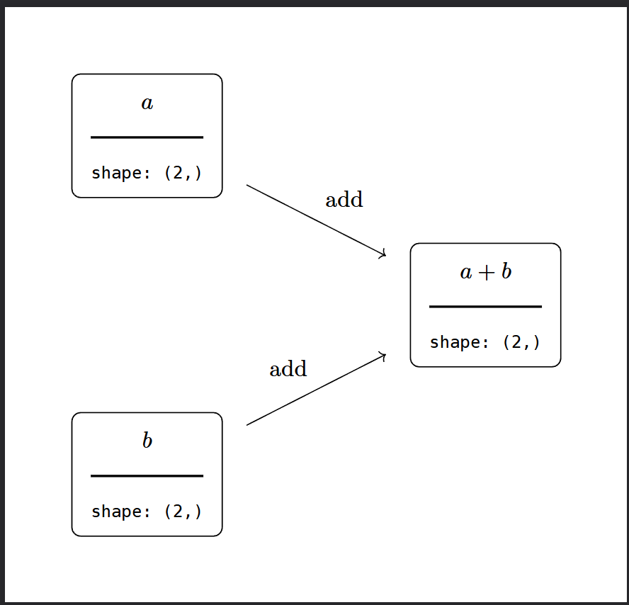
当然, 我们可以修改里面的代码, 比如说绘制一个更复杂的多元函数的链式图

# # Example code
# a = BearTensor("a", np.array([2, 3]))
# b = BearTensor("b", np.array([1, 1]))
# c = a + b
# draw_graph(c, "demo_graph.typ")

a = BearTensor("a", np.array([2, 3]))
b = BearTensor("b", np.array([1, 1]))
c = BearTensor("c", np.array([1, 4]))
d = a * b + b * c + a * c
draw_graph(d, "demo_graph.typ")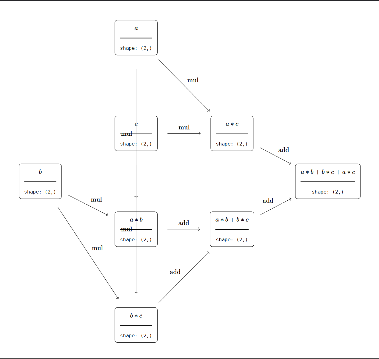

python

Problem 2#

要实现反向传播, 首先要对所有的节点进行拓扑排序, 这样才能搞清楚传播路径

def topological_sort(node):
    '''Return a list of nodes ordered topologically'''

    visited = set()
    sorted_nodes= []
    
    def dfs(current_node):
        if current_node in visited:
            return

        visited.add(current_node)

        for parent_info in current_node.parents:
            dfs(parent_info.parent)

        sorted_nodes.append(current_node)

    dfs(node)
    return sorted_nodes

python

搞清楚这个结点添加的顺序, 举一个简单的例子:

dfs(loss):
  loss 不在 visited → 添加
  遍历 loss.parents → [ReLU]
    dfs(ReLU):
      ReLU 不在 visited → 添加
      遍历 ReLU.parents → [x2]
        dfs(x2):
          x2 不在 visited → 添加
          遍历 x2.parents → [x1]
            dfs(x1):
              +1 不在 visited → 添加
              遍历 +1.parents → [x]
                dfs(x):
                  x 不在 visited → 添加
                  遍历 x.parents → []
                  sorted_nodes.append(x)   ✓
              sorted_nodes.append(x1)      ✓
            sorted_nodes.append(x2)         ✓
          sorted_nodes.append(ReLU)        ✓
      sorted_nodes.append(loss)             ✓

最终: [x, x1, x2, ReLU, loss]

plaintext

这里x是最初的输入, 没有任何依赖, 我们最终需要的梯度就是loss对x的梯度, 为了得到这个梯度, 需要计算一系列loss对中间变量(x1, x2, ReLU)的梯度, 然后通过链式法则得到loss对x的梯度

还需要从某个节点开始, 重置他和他上游(父)节点的所有梯度, 这也需要用递归实现

def reset_children(self):
    """Resets the gradient in the current node to zero and all nodes before it in the computation graph."""
    
    def reset_gradient(node):
        if node.adjoint is not None:
            node.adjoint = 0

        for parent in node.parents:
            reset_gradient(parent.parent)

    reset_gradient(self)

python

现在实现反向传播, 思考一下, 以上面那个例子当中的[x, x1, x2, ReLU, loss], 遍历的顺序应该是从loss开始, 而不是从x开始

遍历到每个节点x, 都需要再遍历x的父节点, 并且更新父节点的梯度

def backward(self):
    """
    Take a node in the computation graph, reset all gradients, and perform backpropagation 
    to compute the adjoints (gradients) for all nodes in the graph.

    Hint: After resetting the gradients, what should the gradient at the current node be?
    """
    self.reset_children()

    sorted_nodes=topological_sort(self)

    sorted_nodes.reverse()

    self.adjoint=1.0

    for node in sorted_nodes:
        
        for parent_info in node.parents:
            parent=parent_info.parent
            grad_fn=parent_info.grad.fn

            parent_grad=grad_fn(node.adjoint)

            parent.adjoint+=parent_grad

python

Problem 3#

实现SGD, Momentum, 实现AdamW优化器

首先考虑优化器的基类, 需要有一个学习率和一堆的参数, 参数是保存为list[BearTensor], value属性保存参数值, adjoint属性保存梯度

class Optimizer:
    def __init__(self, params: list[BearTensor], lr: float):
        self.params = params
        self.lr = lr

    def zero_grad(self):
        for p in self.params:
            p.adjoint = np.zeros_like(p.value)

    def step(self):
        # raise NotImplementedError
        for p in self.params:
            p.value -= self.lr * p.adjoint

python

SGD直接照抄基类就行

class SGD(Optimizer):
    def __init__(self, params: list[BearTensor], lr: float):
        super().__init__(params, lr)

    def step(self):
        
        for p in self.params:
            p.value -= self.lr * p.adjoint
        # pass

python

注意Momentum优化器的公式:

\boxed{ \begin{align*} m_t &= \beta \cdot m_{t-1} + g_t \quad \text{(动量项)} \\[6pt] v_t &= -\eta \cdot m_t \quad \text{(速度/增量)} \\[6pt] w_{t+1} &= w_t + v_t = w_t - \eta \cdot m_t \quad \text{(参数更新)} \end{align*} }

先把这些notation映射到我们类里的属性:

\begin{array}{c|c|c} \text{符号} & \text{代码对应} & \text{含义} \\ \hline g_t & \texttt{p.adjoint} & 当前梯度 \\ m_t & \texttt{momentum\_term} & 动量项 \\ v_t & \texttt{self.velocities[i]} & 速度/参数增量 \\ \beta & \texttt{self.beta} & 动量系数 \\ \eta & \texttt{self.lr} & 学习率 \\ w_t & \texttt{p.value} & 参数值 \end{array}

接下来没有任何难度了, 在step方法里遍历参数然后逐个更新就行

class Momentum(Optimizer):
    def __init__(self, params: list[BearTensor], lr: float, beta: float = 0.9):
        super().__init__(params, lr)
        self.beta = beta
        self.velocities = [np.zeros_like(p.value) for p in self.params]

    def step(self):
        for i, p in enumerate(self.params):
            if self.lr != 0:
                prev_momentum = self.velocities[i] / (-self.lr)
            else:
                prev_momentum = 0
            

            momentum_term = prev_momentum * self.beta + p.adjoint
            

            self.velocities[i] = -self.lr * momentum_term
            

            p.value += self.velocities[i]

python

对Adam优化器也做同样的理解

\boxed{ \begin{align*} \text{1. 一阶矩:} \quad & m_t = \beta_1 \cdot m_{t-1} + (1 - \beta_1) \cdot g_t \\[6pt] \text{2. 二阶矩:} \quad & v_t = \beta_2 \cdot v_{t-1} + (1 - \beta_2) \cdot g_t^2 \\[6pt] \text{3. 偏差校正:} \quad & \hat{m}_t = \frac{m_t}{1 - \beta_1^t}, \quad \hat{v}_t = \frac{v_t}{1 - \beta_2^t} \\[6pt] \text{4. 参数更新:} \quad & w_{t+1} = w_t - \eta \cdot \frac{\hat{m}_t}{\sqrt{\hat{v}_t} + \varepsilon} \end{align*} }

\begin{array}{c|c|c} \text{符号} & \text{代码对应} & \text{含义} \\ \hline g_t & \texttt{p.adjoint} & 当前梯度 \\ m_t & \texttt{self.ms[i]} & 一阶矩估计（动量） \\ v_t & \texttt{self.vs[i]} & 二阶矩估计（方差） \\ \hat{m}_t & \texttt{m\_hat} & 校正后一阶矩 \\ \hat{v}_t & \texttt{v\_hat} & 校正后二阶矩 \\ \beta_1 & \texttt{self.beta1} & 一阶矩衰减系数 (0.9) \\ \beta_2 & \texttt{self.beta2} & 二阶矩衰减系数 (0.999) \\ \varepsilon & \texttt{self.eps} & 防止除零 (1e-8) \\ t & \texttt{self.t} & 时间步 \\ \eta & \texttt{self.lr} & 学习率 \end{array}

class Adam(Optimizer):
    def __init__(
        self,
        params: list[BearTensor],
        lr: float,
        beta1: float = 0.9,
        beta2: float = 0.999,
        eps: float = 1e-8,
    ):
        super().__init__(params, lr)
        self.beta1 = beta1
        self.beta2 = beta2
        self.eps = eps
        self.t = 0
        self.ms = [np.zeros_like(p.value) for p in self.params]
        self.vs = [np.zeros_like(p.value) for p in self.params]

    def step(self):
        self.t+=1
        for i,p in enumerate(self.params):
            self.ms[i]=self.beta1*self.ms[i]+(1-self.beta1)*p.adjoint

            self.vs[i]=self.beta2*self.vs[i]+(1-self.beta2)*((p.adjoint)**2)

            m_hat=self.ms[i]/(1-self.beta1**self.t)
            v_hat=self.vs[i]/(1-self.beta2**self.t)

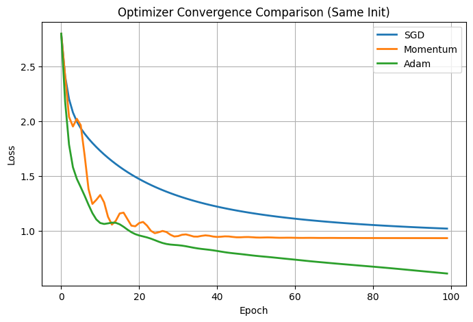
            p.value-=self.lr*m_hat/(np.sqrt(v_hat)+self.eps)

python

运行课程组的代码查看三个优化器的训练曲线

Problem 4#

这里要我们自己写一个训练循环, 唯一要注意的就是把所有的参数注册成BearTensor类, 其他没有什么难点了

from sklearn.datasets import fetch_openml
from sklearn.preprocessing import StandardScaler
from sklearn.model_selection import train_test_split
import numpy as np
import matplotlib.pyplot as plt

# DO NOT CHANGE THE PREPROCESSING CODE
data = fetch_openml("wine-quality-red", as_frame=True)
X = data.data.to_numpy()
y = data.target.to_numpy().astype(float)

scaler = StandardScaler()
X_scaled = scaler.fit_transform(X)

X_train, X_test, y_train, y_test = train_test_split(
    X_scaled, y, test_size=0.4, random_state=42, shuffle=True
)

X_tensor = BearTensor("X_train", X_train)               # shape: (N_train, input_dim)
y_tensor = BearTensor("y_train", y_train.reshape(-1,1)) # shape: (N_train,1)

# Add your training code here!
np.random.seed(42)

input_dim=X_train.shape[1] # 输入维度
hidden_dim=32 # 隐藏层维度
output_dim=1 # 输出维度

W1_init=np.random.randn(input_dim,hidden_dim)*np.sqrt(2.0/input_dim) # 第一个hidden_layer矩阵, input_dim * hidden_dim
W2_init=np.random.randn(hidden_dim,output_dim)*np.sqrt(2.0/input_dim) # 第二个hidden_layer矩阵, hidden_dim * output_dim

W1=BearTensor("W1",W1_init.copy()) # 把参数矩阵注册成为BearTensor类参数
W2=BearTensor("W2",W2_init.copy()) # 同上

params=[W1,W2]  # 注意我们自己实现的Adam类接受的params是一个list[BearTensor]

optimizer=Adam(params,lr=0.01) # 创建优化器, 学习率为0.01

num_epochs=100 # 训练轮数

train_losses=[] # 训练损失
test_losses=[] # 测试损失

for epoch in range(num_epochs):

    optimizer.zero_grad() # 清零梯度

    hidden=(X_tensor@W1).sigmoid() # 前向传播
    output=hidden@W2 # 同上
    
    loss=((output-y_tensor)**2).mean() # 计算损失

    loss.backward()
    optimizer.step() # 更新参数

    train_loss=loss.value.item() # 记录训练损失
    train_losses.append(train_loss) # 记录训练损失     

    # 计算测试损失（不需要梯度）
    X_test_tensor = BearTensor("X_test", X_test)
    y_test_tensor = BearTensor("y_test", y_test.reshape(-1, 1))
    
    # 测试前向传播（使用训练好的权重）
    hidden_test = (X_test_tensor @ W1).sigmoid()
    output_test = hidden_test @ W2
    test_loss = ((output_test - y_test_tensor) ** 2).mean()
    test_losses.append(test_loss.value.item())

    if (epoch + 1) % 10 == 0:
        print(f"Epoch {epoch+1}/{num_epochs}, Train Loss: {train_loss:.4f}, Test Loss: {test_loss.value.item():.4f}")

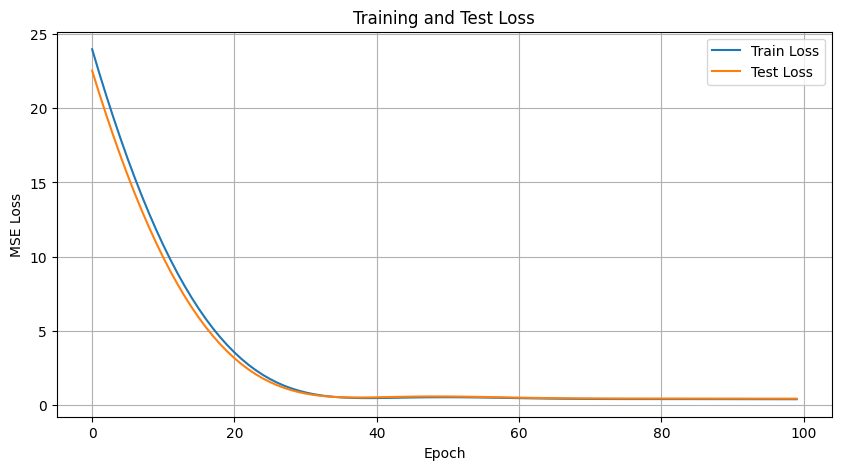
# 打印最终MSE
final_mse = test_losses[-1]
print(f"\nFinal Test MSE: {final_mse:.4f}")

# 绘制损失曲线
plt.figure(figsize=(10, 5))
plt.plot(train_losses, label='Train Loss')
plt.plot(test_losses, label='Test Loss')
plt.xlabel('Epoch')
plt.ylabel('MSE Loss')
plt.title('Training and Test Loss')
plt.legend()
plt.grid(True)
plt.show()

# --- Prediction function ---
def predict(x):
    """Output the scalar prediction for a single training datapoint x"""
    x_tensor=BearTensor("x_input",x.reshape(1,-1))

    hidden=(x_tensor@W1).sigmoid()
    output=hidden@W2

    return output.value.item()
    # pass

python

Epoch 10/100, Train Loss: 11.8084, Test Loss: 10.9215
Epoch 20/100, Train Loss: 4.0232, Test Loss: 3.5952
Epoch 30/100, Train Loss: 0.9623, Test Loss: 0.8673
Epoch 40/100, Train Loss: 0.4591, Test Loss: 0.5058
Epoch 50/100, Train Loss: 0.5181, Test Loss: 0.5702
Epoch 60/100, Train Loss: 0.4653, Test Loss: 0.4989
Epoch 70/100, Train Loss: 0.4054, Test Loss: 0.4402
Epoch 80/100, Train Loss: 0.3933, Test Loss: 0.4299
Epoch 90/100, Train Loss: 0.3896, Test Loss: 0.4261
Epoch 100/100, Train Loss: 0.3834, Test Loss: 0.4217

Final Test MSE: 0.4217

plaintext

UC Berkeley CS189 Assignment 3

CS189 Assignment 3#

项目描述#

例子: 多元微分#

Problem 1#

Problem 2#

Problem 3#

Problem 4#