CS189 Assignment 2#
项目描述#
书接上回, 这个lab里我们主要关心两个问题:
- 如何对模型的能力建模, 即如何通过PK当中模型的输赢情况以及一些潜在的其他特征, 通过逻辑回归的方式给每个模型一个能力分数
- 新特征对模型能力的影响, 如果加入一些额外的特征, 模型的排名会发生什么变化
Part1代码复用#
这里要用到subselect_battles函数, 直接从part1复制过来就行, 不再赘述了
Problem 4#
概率建模#
我们希望先搞一个LeaderBoard, 对于每一个模型m, 能给他一个”strength score” , 这个score能反应:
-- score的排名反映了此模型对战另一个模型时的胜率

-- 量化的看, 对于模型A和B, A战胜B的概率应该是$$S_A - S_B$$的函数换言之, 我们希望找到一个函数使得:
比如说用sigmoid函数:
本质上这就是学习一个logistic regression
数据结构设计#
可以把一行数据表示为这种数据结构:
-- 一个feature vector表示两个model

-- 一个label表示胜出的模型举个例子, 原始的行为:
row = {'model_a': 'gpt-4o-2024-05-13', 'model_b': 'claude-3-opus-20240229', 'winner': 'model_a'}`可表述为这两行(两行是因为PK是相互的, A赢了B同时也代表B赢了A)
Feature 1:[1, -1]
Label: 1index 0 表示gpt, index 1表示claude, 1表示gpt胜出
Feature 2:[-1, 1]
Label: 0index 0 表示gpt, index 1表示claude, 0表示claude未胜出
通俗一点的说就是如果Label是站在feature = 1的视角来看的, 如果1赢了-1, 那么Label就是1, 如果1输了, 那么Label就是0
为什么同一行要解释成两个不同的feature vector呢? 对于含有A,B模型的一行, 我们可能要建模
显然这两个feature vector就是[S_A - S_B, S_B - S_A]的系数矩阵
多个模型的情况#
假如有多个模型, 也只不过是把所有的Feature Vector和Label(以前面那种方法得到的)组成X和y而已
比如说有5个模型
索引:    0         1          2        3         4
模型: [GPT-4o, Claude-3, Gemini, Llama-3, PaLM-2]如果GPT赢了Claude, 那么对应的Feature Vector和Label应该是
[+1, 0, 0, -1, 0], 1
[-1, 0, 0, +1, 0], 0没参加PK的模型的值赋为0即可
Problem 4a#
遍历每一行, 对于每一行再去遍历所有的models, 遍历到model_a就记为1, model_b就记为-1, 其他的就记为0, 再根据winner打个标就行
def turn_into_features(df, models):
    '''
    Convert pairwise battle results into feature matrix X and label vector y
    suitable for logistic regression based on the Bradley-Terry model
    '''
    # TODO:
    # 1. Iterate through each row in the DataFrame.
    # 2. For each battle, create a feature vector:
    #    - Assign +1 to the column corresponding to 'model_a'.
    #    - Assign -1 to the column corresponding to 'model_b'.
    #    - All other columns should be 0.
    # 3. Append the label:
    #    - 1 if 'model_a' is the winner.
    #    - 0 if 'model_b' is the winner.
    # 4. Return the feature matrix X and label vector y as numpy arrays.
    X = []
    y = []


    for _ ,row in df.iterrows():
        a=row['model_a']
        b=row['model_b']

        win_a=1 if row['winner']==a else 0

        x_ab=[1 if col==a else -1 if col==b else 0 for col in models]

        y_ab=win_a

        x_ba=[1 if col==b else -1 if col==a else 0  for col in models]

        y_ba=1-win_a

        X.append(x_ab)
        y.append(y_ab)
        X.append(x_ba)
        y.append(y_ba)
    return np.array(X), np.array(y)

X, y = turn_into_features(selected_battles_no_ties, selected_models)
X.shape, y.shape注意为什么两个y是互斥的, 因为都是站在每一个feature = 1的视角去看, 如果第一个feature = 1赢了-1, 那么第二个feature = 1肯定就输了, 所以一定是互斥的
Xarray([[ 0, 0, 0, ..., 0, 0, -1],
[ 0, 0, 0, ..., 0, 0, 1],
[ 0, 0, 0, ..., 0, 1, 0],
...,
[-1, 0, 0, ..., 0, 0, 0],
[ 0, 0, 0, ..., 0, 0, 0],
[ 0, 0, 0, ..., 0, 0, 0]], shape=(51066, 20))这个标签的设计是合理的, 假设feature vector是[1,-1]而A赢了, 那么label是1, 此时当然也希望是接近于1的
Problem 4b#
用LogisticRegression来训练即可
from sklearn.linear_model import LogisticRegression


model = LogisticRegression(fit_intercept=False)
scores = model.fit(X,y).coef_[0]

results = {"Model": selected_models, "Score": scores}
results_df = pd.DataFrame(results).sort_values("Score", ascending=False).reset_index(drop=True)
results_df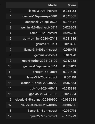
解释一下为什么对于两个模型A和B, 输出
就代表A战胜B的概率, 这和我们之前设计的特征工程有关, 比如说训练集上所有情况下A都战胜了B, 那么feature vector和label都为[1,-1]和1, 也就是说训练得到的[w_1, w_2]大概率会满足
由于特征工程的设计,权重向量 中的每个元素 就是模型 的 strength 。因此 直接给出了 A 战胜 B 的预测概率。
Problem 5a#
我们要用重采样的方式来重复训练逻辑回归模型, 每个逻辑回归模型会给我们这些LLM一组分数, 在得到许多组分数之后, 我们就可以得到每个LLM的分数和置信区间
举个例子, 每次训练完成之后, 逻辑回归模型会给gpt4o这个模型一个分数, 假如我们训练了一百次逻辑回归, 那就会有一百个分数, 我们可以取这个分数的均值, 还可以取2.5%分位数和97.5%分位数, 得到置信区间
def get_bootstrapped_score(X, y, models, category_name="Overall", n_bootstrap=10):
    """
    Bootstraps logistic regression model scores to estimate confidence intervals.
    Args:
        X: Feature matrix
        y: Labels
        models: List of model names (order matches columns of X)
        n_bootstrap: Number of bootstrap samples
    Returns:
        results_df: DataFrame with Model, Average Score, Lower Bound, Upper Bound
        mean_scores: Mean of bootstrapped scores (np.array)
        confidence_intervals: 2.5 and 97.5 percentiles (np.array shape [2, n_models])
    """
    #TODO

    np.random.seed(189)  # for reproducibility
    bootstrap_scores = []
    for i in range(n_bootstrap):
        indices = np.random.choice(len(X), size=len(X), replace=True)
        X=X[indices]
        y=y[indices]
        model = LogisticRegression(fit_intercept=False)
        model.fit(X,y)
        bootstrap_scores.append(model.coef_[0])
    bootstrap_scores = np.array(bootstrap_scores)
    mean_scores = bootstrap_scores.mean(axis=0)
    confidence_intervals = np.percentile(bootstrap_scores, [2.5, 97.5], axis=0)

    results = {
        "Model": models,
        "Average Score": mean_scores,
        "Lower Bound": confidence_intervals[0],
        "Upper Bound": confidence_intervals[1],
        "Category": category_name,
    }
    results_df = pd.DataFrame(results)
    return results_df, mean_scores, confidence_intervals
results_df, mean_scores, confidence_intervals = get_bootstrapped_score(X, y, selected_models, n_bootstrap=10)

# Test that confidence intervals make sense
assert (confidence_intervals[0] <= confidence_intervals[1]).all(), "Every lower bound must be <= upper bound."
assert ((confidence_intervals[0] <= mean_scores) & (mean_scores <= confidence_intervals[1])).all(), "Each mean score should lie within its CI."代码写起来也简单, 只要注意一下np.percentile的用法就行
可视化每个模型的置信区间:
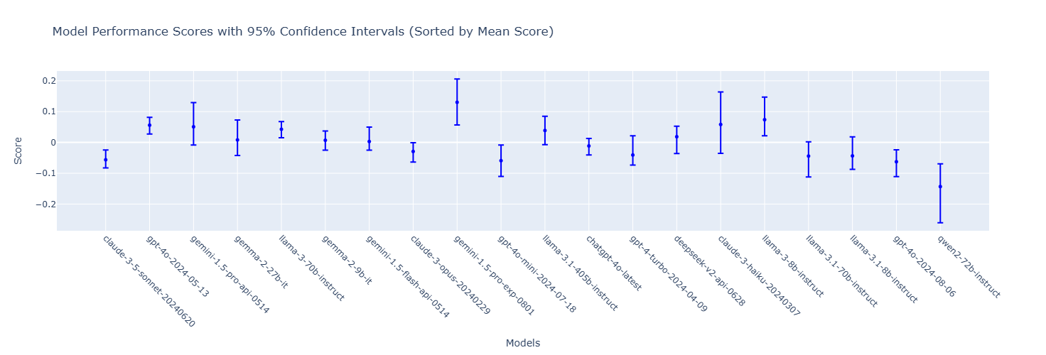
在之前的单次实验当中, 虽然llama-3-70b-instruct的分数最高, 但是从这个图看来, 最好的应该是gemini-1.5-pro-exp-0801(我主观上也这么认为)
Problem 5b#
有了置信区间, 我们可以比较保守的给出一个A模型好于B模型的定义, 即若A的Lower Bound大于B的Upper Bound, 那么我们就认为A好于B, 我们可以根据这个规则给出rank
注意这里的代码需要遍历两次, 对于每个模型, 还要遍历除了他之外的所有模型, 逐个比较强弱关系, 我们用count来记录A模型超过了多少其他模型, 注意这个条件十分严格, 一定要置信区间下界大于其他模型的上界才行
def assign_rank(row, df=results_df):
    """
    Input:
        row : pd.Series
            A row of the DataFrame (representing a model’s metrics).
        df : pd.DataFrame (default = results_df)
            DataFrame containing model performance with 'Lower Bound' and 'Upper Bound'.

    Output:
        int : The rank of the model, defined as (# of models confidently better) + 1.
    """

    count = 0
    for _,row2 in df.iterrows():
        if row['Lower Bound'] > row2['Upper Bound']:
            count+=1

    return count


results_df['Rank'] = results_df.apply(lambda r: assign_rank(r, results_df), axis=1)
results_df = results_df.sort_values(by="Rank", ascending=True)
results_df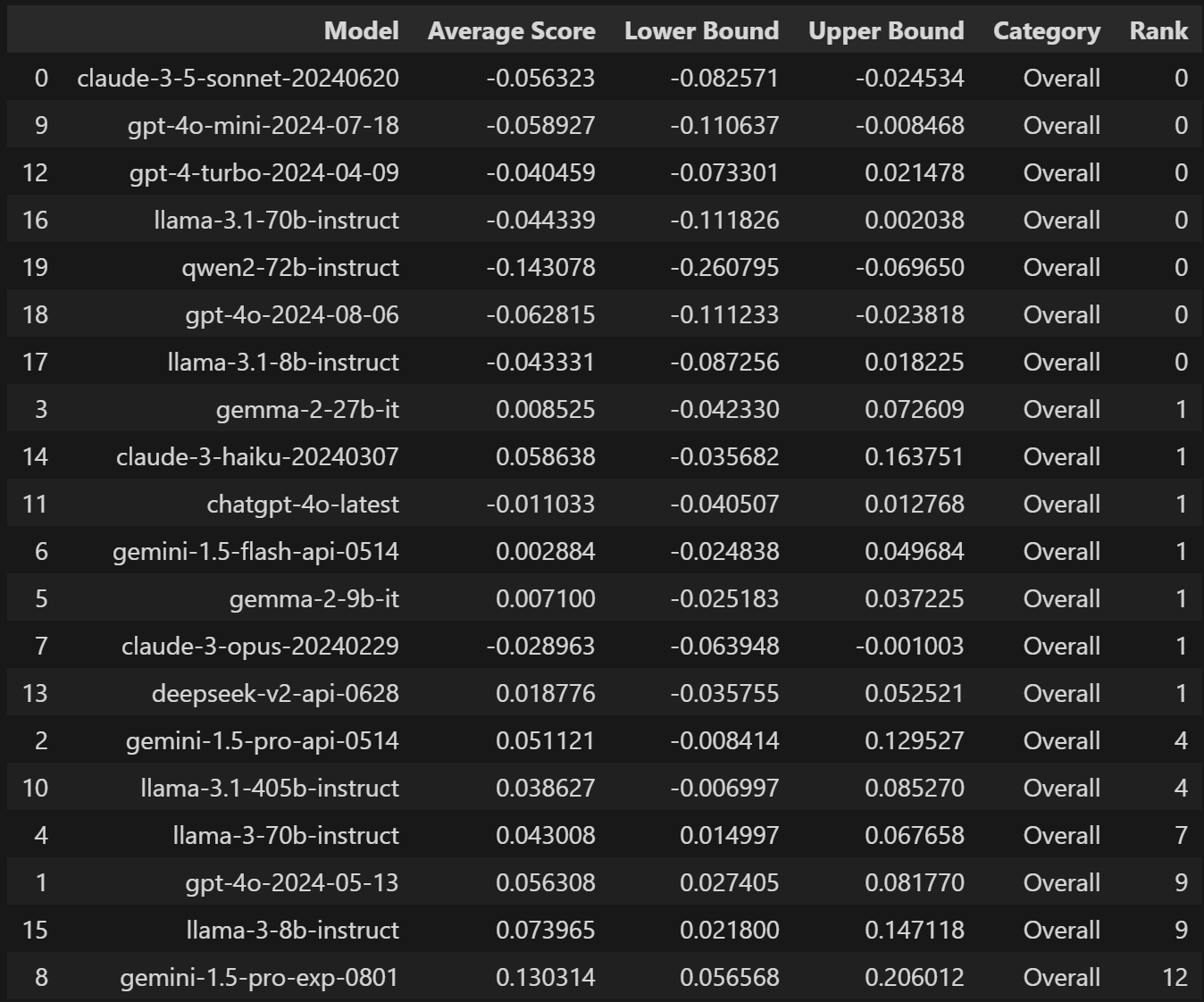
注意结果上有很多比较好的模型都并列rank = 0了
Problem 7a#
假设我们现在收到的对话语料的格式为:
conv_example = {
    "conversation": [
        {"role": "user", "content": "How do I sum a list in Python?"},
        {"role": "assistant", "content": "Use the built-in function: sum(your_list)."}
    ]
}需要计算所有role == assistant的content的token长度, 这里题目告诉我们调用gpt2的分词器即可
import tiktoken
def calculate_response_length(conv):
    enc=tiktoken.get_encoding('gpt2')

    assistant_contents=[msg['content'] for msg in conv['conversation'] if msg['role']=='assistant']

    joined_text="\n\n".join(assistant_contents)

    tokens=enc.encode(joined_text,disallowed_special=())

return len(tokens)先按照条件筛选, 然后把每条句子join起来, 用分词器编码之后返回长度即可
Problem 7b#
回忆一下我们的PK数据的格式, 每一行当中有这四列:
model_a model_b conversation_a conversation_b现在希望把model_a和conversation_a分出来, 计算一下conversation_a的token长度(用7a实现的那个函数), 对conversation_b也做同样的操作, 然后竖着concat起来, 相当于以前有n行, 处理之后变成2n行了
#TODO:
battles_a = selected_battles_no_ties[['conversation_a','model_a']].rename(columns={'conversation_a':'conversation','model_a':'model'})

battles_a['response_length']=battles_a['conversation'].apply(lambda c:calculate_response_length({'conversation':c}))

battles_b = selected_battles_no_ties[['conversation_b','model_b']].rename(columns={'conversation_b':'conversation','model_b':'model'})

battles_b['response_length']=battles_b['conversation'].apply(lambda c:calculate_response_length({'conversation':c}))

per_model_battles=pd.concat([battles_a,battles_b])
per_model_battles.head()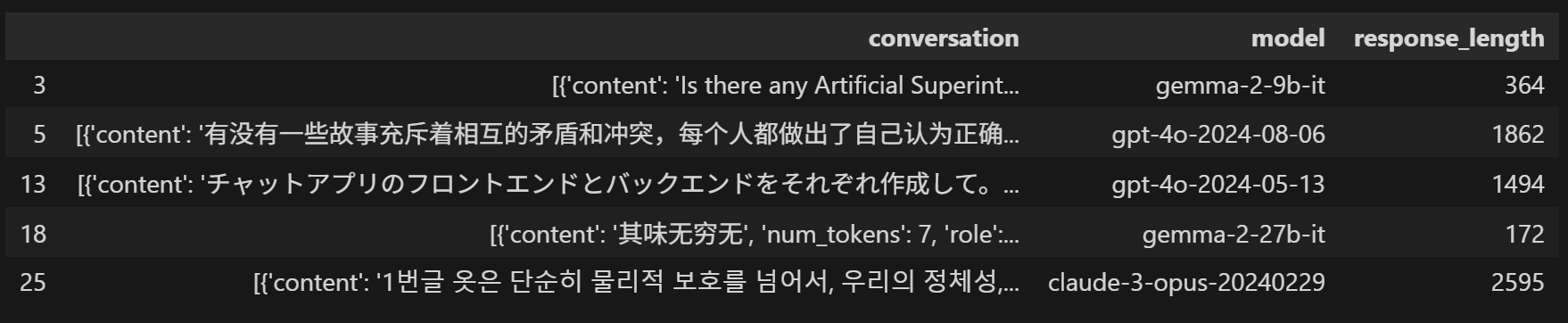
注意这个conversation是个比较复杂的嵌套结构, 可以理解为他是一个list, 当中的每一个值是User/Assistant说的一句话
[{'content': 'Is there any Artificial Superintelligence?', 'num_tokens': 7, 'role': 'user'}
 {'content': "As a large language model, I am not able to provide an opinion or belief on whether or not artificial superintelligence exists. The concept of artificial superintelligence is a topic of much debate and speculation.\n\nHere's what we know:\n\n* **Current AI:** Today's AI, including myself, is very good at specific tasks, like generating text, translating languages, and playing games. However, we lack the general intelligence and common sense of humans.\n* **Superintelligence Definition:** Artificial superintelligence is generally defined as an AI that surpasses human intelligence in all aspects. This includes things like problem-solving, creativity, and learning.\n* **No Consensus:** There is no scientific consensus on whether or not artificial superintelligence is possible or even desirable. Some experts believe it is inevitable, while others believe it is highly unlikely or even dangerous.\n\nThe development of artificial superintelligence is a complex and multifaceted issue with profound implications for society. It is important to continue to have open and honest discussions about the potential benefits and risks of this technology.", 'num_tokens': 208, 'role': 'assistant'}
 {'content': 'What is your knowledge cutoff date?', 'num_tokens': 7, 'role': 'user'}
{'content': "I can access pretty up-to-date information, which means I don't really have a knowledge cut-off date. However, keep in mind:\n\n* **I am not constantly updating:** I don't have real-time information like a search engine. My knowledge is based on the massive dataset I was trained on.\n\n* **Training data has a limit:** That training dataset does have a point in time when it was last updated. While it's extensive, there will always be newer information I'm not aware of.\n\nSo, while I strive to be as current as possible, it's best to double-check anything time-sensitive with a reliable source.", 'num_tokens': 127, 'role': 'assistant'}]按照之前得到的LLM的rank顺序, plot每个模型的token长度:
model_lineup = results_df.sort_values("Rank")['Model'].tolist()
avg_lengths = per_model_battles.groupby("model")["response_length"].mean().reset_index()
avg_lengths["model"] = pd.Categorical(avg_lengths["model"], categories=model_lineup, ordered=True)
avg_lengths = avg_lengths.sort_values("model").reset_index(drop=True)

# Add a numeric rank column for trendline fitting
avg_lengths["rank"] = avg_lengths.index + 1  # 1 = best, etc.

# Fit a linear trendline (polyfit) to the response length vs. rank
z = np.polyfit(avg_lengths["rank"], avg_lengths["response_length"], 1)
p = np.poly1d(z)
trendline = p(avg_lengths["rank"])

fig = go.Figure()

fig.add_trace(go.Scatter(
    x=avg_lengths["model"],
    y=avg_lengths["response_length"],
    mode='lines+markers',
    name='Avg Response Length'
))

fig.add_trace(go.Scatter(
    x=avg_lengths["model"],
    y=trendline,
    mode='lines',
    name='Trendline',
    line=dict(dash='dash', color='red')
))

fig.update_layout(
    title="Average Response Length of Models (with Trendline)",
    xaxis_title="Model (sorted by performance)",
    yaxis_title="Average Response Length",
    xaxis_tickangle=45,
    yaxis=dict(range=[0, max(avg_lengths["response_length"].max(), trendline.max()) * 1.05])  # y-axis starts at 0
)

fig.show()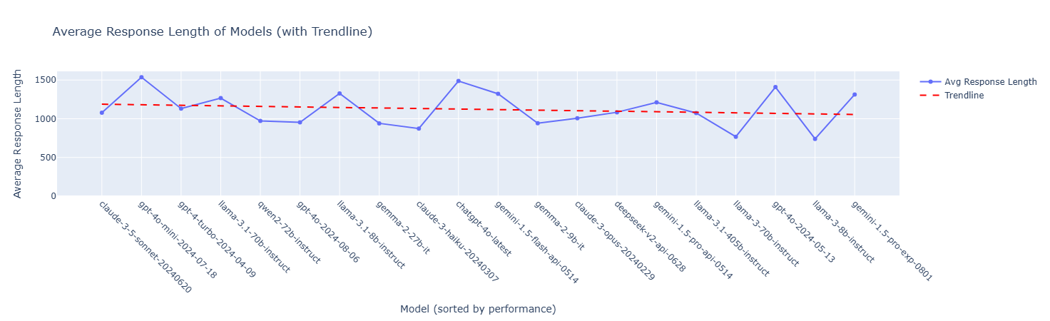
可以看出模型好坏和对话的token长度并无直接关系
Problem 8a#
从conv_metadata字段当中拿到一些额外的特征, 先给出一个正则化函数normdiff, 相当于计算出两个model的某一个特征得分之差
先看一下在这个嵌套字段conv_metadata当中有什么
selected_battles_no_ties['conv_metadata'].iloc[0]{'bold_count_a': {'**': 5, '__': 0},
'bold_count_b': {'**': 0, '__': 0},
'context_a_tokens': 222,
'context_b_tokens': 230,
'header_count_a': {'h1': 0, 'h2': 0, 'h3': 0, 'h4': 0, 'h5': 0, 'h6': 0},
'header_count_b': {'h1': 0, 'h2': 0, 'h3': 0, 'h4': 0, 'h5': 0, 'h6': 0},
'list_count_a': {'ordered': 0, 'unordered': 5},
'list_count_b': {'ordered': 0, 'unordered': 0},
'sum_assistant_a_tokens': 335,
'sum_assistant_b_tokens': 287,
'sum_user_tokens': 14,
'turns': 2}总之就是定义了一些特征, 然后分别在两个model上去计算这些特征, 需要注意的一点是, 特征的计算方式是求和计算, 比如说我想通过blod_count_a计算得到bold_a, 那在上面这个例子上应该是5+0=5
def add_style_features(df):
    """
    Adds normalized style feature difference columns to the DataFrame.
    The columns added are:
      - style_bold_count
      - style_header_count
      - style_list_count
      - style_sum_assistant_tokens
    """
    def normdiff(a, b):
        denom = a + b
        return 0 if denom == 0 else (a - b) / denom


    style_bold = []
    style_header = []
    style_list = []
    style_tokens = []
    for idx, row in df.iterrows():

        meta=row['conv_metadata']

        bold_a=sum(meta['bold_count_a'].values())
        bold_b=sum(meta['bold_count_b'].values())

        header_a=sum(meta['header_count_a'].values())
        header_b=sum(meta['header_count_b'].values())

        list_a=sum(meta['list_count_a'].values())
        list_b=sum(meta['list_count_b'].values())

        tokens_a=meta['sum_assistant_a_tokens']
        tokens_b=meta['sum_assistant_b_tokens']

        style_bold.append(normdiff(bold_a,bold_b))
        style_header.append(normdiff(header_a,header_b))
        style_list.append(normdiff(list_a,list_b))
        style_tokens.append(normdiff(tokens_a,tokens_b))


    df["style_bold_count"] = style_bold
    df["style_header_count"] = style_header
    df["style_list_count"] = style_list
    df["style_sum_assistant_tokens"] = style_tokens
    return df

# Example usage:
selected_battles_no_ties = add_style_features(selected_battles_no_ties)Problem 8b#
接下来我们要重构一下数据的格式, 把原来的一行拆成两行, 例如

这应该比较简单, 别忘了我们已经有了style_feature_cols那些字段, 我们只要和之前一样做出X,y和direction, 然后for循环style_feature_cols拿到我们刚才通过norm_diff计算的一些额外特征就行了
def make_pairwise_feature_df(df, models, style_feature_cols):
    """
    For each row in df, create two rows in the output:
      - One for A->B (original direction)
      - One for B->A (flipped direction)
    Each row contains:
      - question_id
      - X: model indicator vector (1 for model_a, -1 for model_b, 0 otherwise)
      - y: 1 if model_a wins, 0 if model_b wins
      - style features (from style_feature_cols)
      - direction: "A->B" or "B->A"
    Returns a new DataFrame with only these columns.
    """
    ...
    records = []
    for idx, row in df.iterrows():
        # X vector for A->B and B->A
        x_a_b=[1 if row['model_a']==model else -1 if row['model_b']==model else 0 for model in models]
        x_b_a=[-1 if row['model_a']==model else 1 if row['model_b']==model else 0 for model in models]
        # y for A->B and B->A
        y_a_b=1 if row['winner']=='model_a' else 0
        y_b_a=1 if  y_a_b==0 else 1
        # Style features for A->B, B->A
        style_ab=row[style_feature_cols].to_numpy(dtype=float)
        style_ba=-style_ab

        rec_a={
          "question_id":row['question_id'],
          "X":x_a_b,
          "y":y_a_b,
          "direction":"A->B",
        }

        for col,val in zip(style_feature_cols,style_ab):
          rec_a[col]=val

        rec_b={
          "question_id":row['question_id'],
          "X":x_b_a,
          "y":y_b_a,
          "direction":"B->A",
        }

        for col,val in zip(style_feature_cols,style_ba):
          rec_b[col]=val


        # Add A->B, B->A
        records.append(rec_a)
        records.append(rec_b)


    return pd.DataFrame(records)

style_feature_cols = [
    "style_bold_count",
    "style_header_count",
    "style_list_count",
    "style_sum_assistant_tokens"
]

pairwise_feature_df = make_pairwise_feature_df(selected_battles_no_ties, selected_models, style_feature_cols)
pairwise_feature_df.head(2)Problem 8c#
根据上面的图, 现在我们有了一些额外的特征, 我们把这些额外的特征接到X向量的后面, 相当于得到了一些额外的feature
唯一的难点在于特征的拼接, 我们需要先把原来的X列通过hstack竖着拼接成二维数组, 然后把额外特征列to_numpy成二位数组, 再用hstack水平拼接起来
参考以下这个可视化变换:
# 假设 df['X'] 是这样的:
# 0    [1, -1, 0, 0]
# 1    [0, 1, -1, 0]
# 2    [-1, 0, 1, 0]

X_id = np.vstack(df['X'].values)
# 结果:
# array([[ 1, -1,  0,  0],
#        [ 0,  1, -1,  0],
# [-1, 0, 1, 0]])# style_features = ['style_bold_count', 'style_header_count', ...]
X_style = df[style_features].to_numpy()
# 结果:
# array([[ 0.5, 0.2, 0.3, 0.1],
# [ 0.1, 0.8, 0.2, 0.4],
# [ 0.3, 0.1, 0.5, 0.2]])X_with_style = np.hstack([X_id, X_style])
# 结果:
# array([[ 1, -1, 0, 0, 0.5, 0.2, 0.3, 0.1],
# [ 0, 1, -1, 0, 0.1, 0.8, 0.2, 0.4],
# [-1, 0, 1, 0, 0.3, 0.1, 0.5, 0.2]])
#
# 前4列 = 模型标识特征 (X_id)
# 后4列 = 风格特征 (X_style)┌─────────────────────────────────────────────────────────────┐
│ 水平拼接 np.hstack │
├──────────────────────┬────────────────────────────────────┤
│ X_id (模型标识) │ X_style (风格特征) │
│ (4列: 1/-1/0) │ (4列: normdiff计算的值) │
│ │ │
│ [ 1, -1, 0, 0 | 0.5, 0.2, 0.3, 0.1] │
│ [ 0, 1, -1, 0 | 0.1, 0.8, 0.2, 0.4] │
│ [-1, 0, 1, 0 | 0.3, 0.1, 0.5, 0.2] │
└──────────────────────┴────────────────────────────────────┘
↓
最终特征矩阵 X_with_style
shape = (n_samples, 8)def get_sc_category_results(df, selected_models, filter_mask = None,
category_name="Overall w/ Style Control",
n_bootstrap=10, style_features=style_feature_cols):
feature_labels = selected_models + style_features
if filter_mask is not None:
df = df[filter_mask]
X_id = np.vstack(df['X'].values)
X_style = df[style_features].to_numpy()
X_with_style = np.hstack([X_id, X_style])
results_df, mean_scores, confidence_intervals = get_bootstrapped_score(
X_with_style, df["y"].to_numpy(), feature_labels,
category_name=category_name, n_bootstrap=n_bootstrap
)
results_df["Rank"] = results_df.apply(lambda r: assign_rank(r, results_df), axis=1)
results_df.loc[results_df["Model"].isin(style_features), "Rank"] = -1
# 按题目要求重新排列顺序
cols = ['Model', 'Category', 'Average Score', 'Lower Bound', 'Upper Bound', 'Rank']
results_df = results_df[cols]
return results_df
results_df_style_control = get_sc_category_results(
pairwise_feature_df, selected_models,
category_name="Overall w/ Style Control", n_bootstrap=10
)
combined_results_df = pd.concat([results_df, results_df_style_control], ignore_index=True)
cols = ['Model', 'Category', 'Average Score', 'Lower Bound', 'Upper Bound', 'Rank']
combined_results_df = combined_results_df[cols]
fig = plot_rank_heatmap(combined_results_df, title="With and Without Style Control")
fig.show()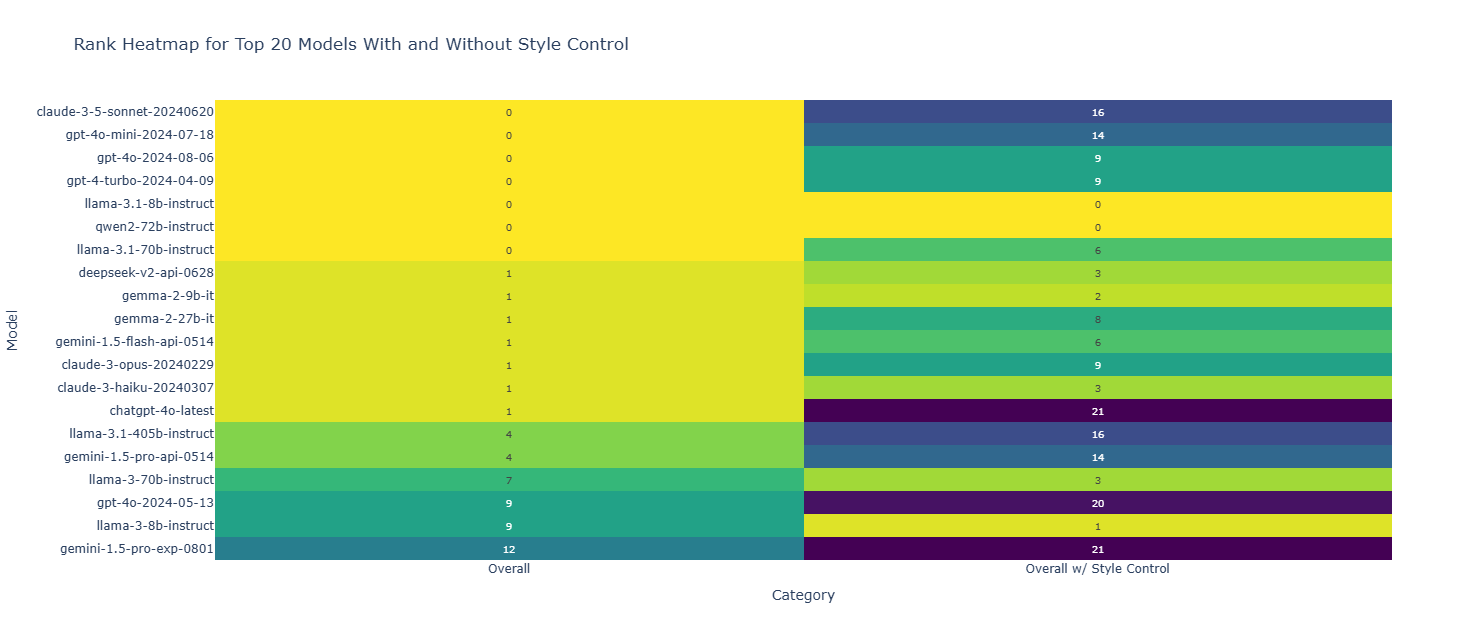
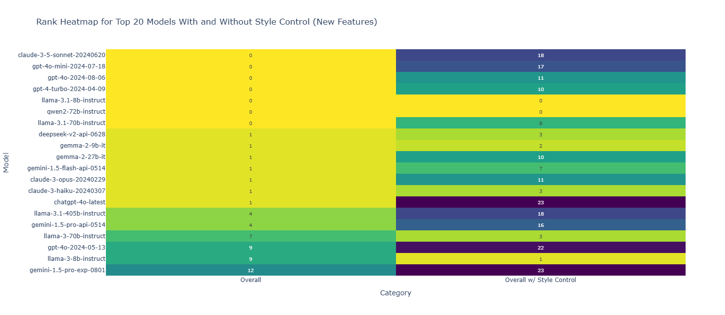
在加入了一些特征之后, 模型的排名发生了很大变化
Problem 9a#
课程组给出了计算TF-IDF的代码, 这段代码能够计算出一个phrase在llama-3.1的回答中的”常用程度”和在其他模型当中的”常用程度”, 运行这些代码得到示例结果:
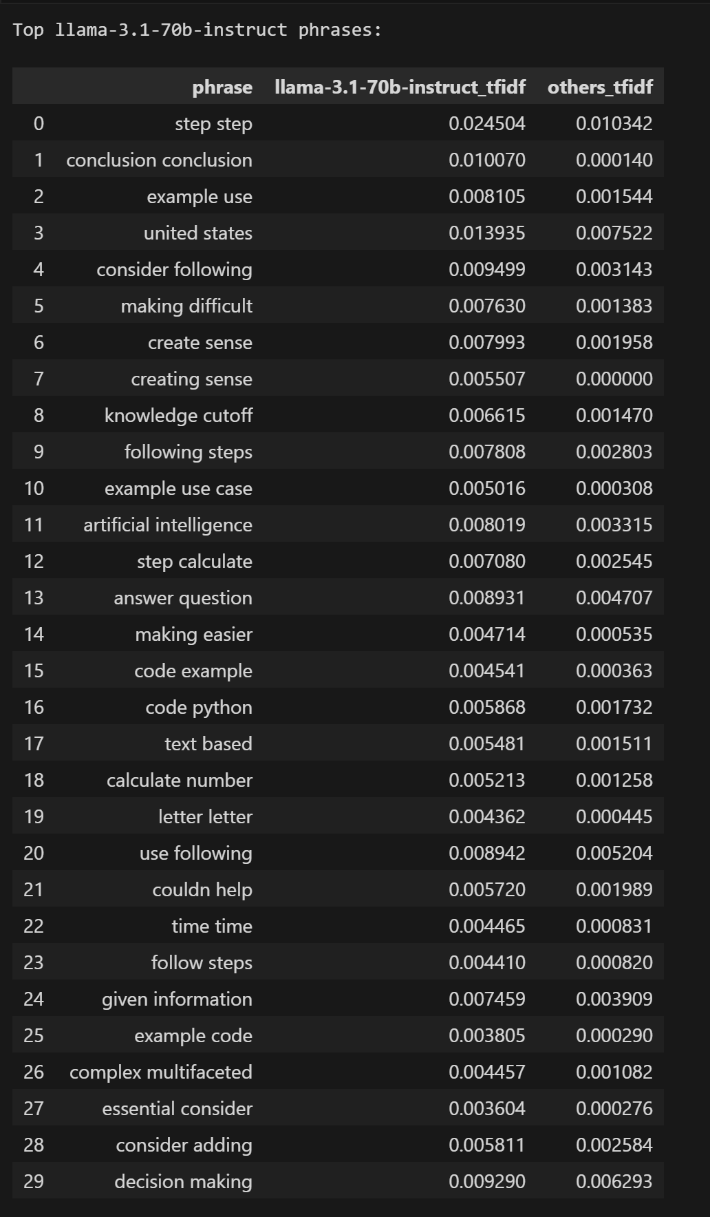
表里面每个词都是在llama-3.1的回答中出现的比较频繁, 而在其他模型的回答中出现的很少的词
现在的任务是从原始数据出发, 只考虑英语的对话, 然后把他们拆成两部分, 一部分是winner == model_a的行, 一部分是winner == model_b的行, 调用给出的tfidf_phrase_diff函数得到表即可, 这个表的含义就是那些在model_a赢的回答中出现多的词或反之
# TFIDF comparing winning responses to losing responses
...
# 1) Restrict to English Only and prepare assistant-only strings for A/B
# Use 'convert_asst_conversation_to_string' helper function
selected_battles_english = selected_battles_no_ties[selected_battles_no_ties['language'] == 'English'].copy()

selected_battles_english['asst_a']=selected_battles_english['conversation_a'].apply(convert_asst_conversation_to_string)
selected_battles_english['asst_b']=selected_battles_english['conversation_b'].apply(convert_asst_conversation_to_string)

# 2) Build lists of assistant-only winning/losing responses
winning_responses = selected_battles_english.apply(lambda row:row['asst_a'] if row['winner']=='model_a' else row['asst_b'],axis=1).tolist()

losing_responses = selected_battles_english.apply(lambda row:row['asst_a'] if row['winner']=='model_b' else row['asst_b'],axis=1).tolist()

# 3) Compare phrases
df_win, df_lose = tfidf_phrase_diff(winning_responses, losing_responses, "winning", "losing")
# 4) Show results
print("Top winning response phrases:")
display(df_win)
print("Top losing response phrases:")
display(df_lose)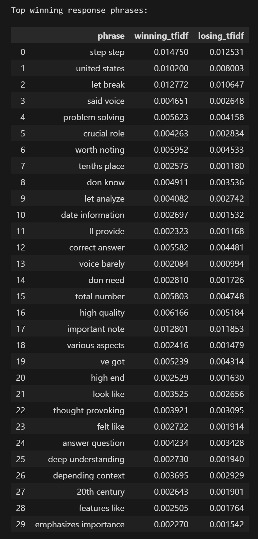
Problem 9b#
开放性问题, 要我们自己挖一个特征出来, 这里我选的是手动添加一些词, 然后遍历每行的conversation_a和conversation_b去看是否包含这些词当中的任意词语, 就可以得到两个bool变量, 最后相减得到新特征
# Design your own stylistic feature(s) that compare model A vs B on each row.
# Keep it simple (boolean presence, counts, or normalized differences) or get creative.

# Remember might want to normalize difference, if you compute counts

# TODO: Define your feature function
def YOUR_FUNC(row):
    #Input: a row with 'conversation_a' and 'conversation_b' (each is a list of {role, content} dicts).
    #Output: a single numeric feature comparing A vs B (e.g., -1/0/1, count diff, or normalized diff).
    #Hint: You probably want to inspect only assistant messages.
    # Example (placeholder): return 0
    phrases = [
        "step by step",
        "follow these steps",
        "the following steps",
        "let's break it down",
        "let us break it down",
        "for example",
        "for instance",
        "in summary",
        "to summarize"
    ]
    a_has=False
    b_has=False

    for msg in row['conversation_a']:
        if msg['role'] == 'assistant':
            text = msg['content'].lower().replace("-", " ")
            if any([p in text for p in phrases]):
                a_has=True
    for msg in row['conversation_b']:
        if msg['role'] == 'assistant':
            text = msg['content'].lower().replace("-", " ")
            if any([p in text for p in phrases]):
                b_has=True

    return int(a_has)-int(b_has)

# TODO: Apply your function to create a new column
selected_battles_no_ties.loc[:, "YOUR_FEATURE"] = selected_battles_no_ties.apply(YOUR_FUNC, axis=1)

# Choose which style features to control for in ranking.
# Start from this list and add yours below.
style_feature_cols = [
    "style_bold_count",
    "style_header_count",
    "style_list_count",
    "style_sum_assistant_tokens",
    "refusal_count",
    "YOUR_FEATURE",   # <- uncomment after you create it
]

pairwise_feature_df = make_pairwise_feature_df(selected_battles_no_ties, selected_models, style_feature_cols)

combined_results_df_new = get_sc_category_results(pairwise_feature_df,
                                 selected_models,
                                 category_name="Overall w/ Style Control",
                                 n_bootstrap=10,
                                 style_features=style_feature_cols)

fig = plot_rank_heatmap(pd.concat([results_df, combined_results_df_new]), title="With and Without Style Control (New Features)", selected_models=selected_models)
fig.show()

# Create and display the plot
fig = plot_style_features(combined_results_df_new, selected_models)
fig.show()